Floyd Warshalls algorithm

In this chapter we shall learn about below topics:

In this tutorial we shall learn about Floyd warshalls algorithm. This algorithm is used to find shortest path from all the vertices to every other vertex. This is the 3rdtype to find shortest path between source node to destination node.

We shall solve this by using dynamic programming approach.

Before going to study Floyd warshalls algorithm, let’s review previous 2 algorithms.

1. Dijkstra’s algorithm: This algorithm is used when we need to find shortest path from one node to all the other nodes/vertices.

2. Bellman Ford Algorithm: This algorithm is used to find shortest path from one node to all the other nodes, -ve edges are allowed.

3. Floyd Warshalls algorithm: This algorithm is used to find all the shortest path from all the vertex to every other vertex. Here also –ve valued edges are allowed.

As said earlier, the algorithm uses dynamic programming to arrive at the solution. So DP approach as we saw in earlier chapter, uses memorization technique and divide the problem into simple sub problems and solve those sub problems to arrive at the solution.

Consider the below graph:

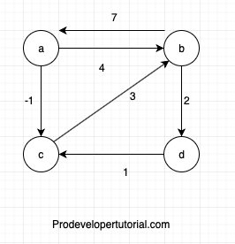
From the above graph, calculate the distance matrix.

While constructing a distance matrix, if there is a direct edge between 2 nodes then write the value. If there is no direct path then make it as Infinity.

Below will be the distance matrix. We shall name it as “D0”.

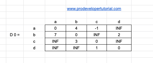
As you can see from the above matrix, the diagonal value is always zero. This is because the cost of source to destination form the same node is zero.

As there are 4 vertices, we need to create 4 matric table. One for each node. Hence at the end we get the shortest path from any vertex to any other vertex.

As we are using DP approach, we shall take help of previously generated matrix and calculate the values based on that.

Now let’s write D1 matrix. For D1 matrix, we take 1strow and 1stcolumn from D0 matrix. Initial D1 matrix is as below:

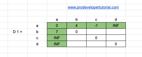
To fill D1 matrix we shall take help of D0 matrix as reference.

Now we dill the remaining empty cells. To fill that we use below 2 steps:

1. Check if there is a direct path from source to destination vertex. If there is, make a note of it.

2. Check if there is a path via the node that we are currently in use. If there is a path, make a note of the total distance via the current node.

Then take the min value of above 2 values and fill in the matrix.

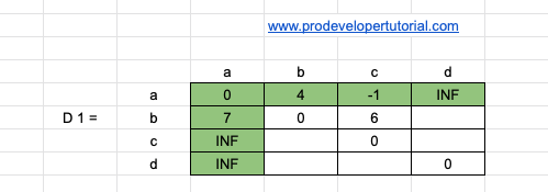
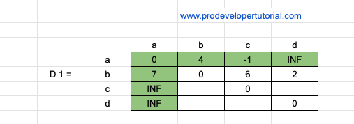
For our current matrix D1, we must need to fill [b, c] and [b, d]. Here we shall take D0 matrix as reference and fill D1 matrix.

1. [b, c] => Check if there is a direct path from D0 matrix. No there is not. Now check if there is a path including “a” i.e “b -> a, a -> c”.

There is and the cost is “ 7 -1 = 6”. This is less than INF.

Update the matrix

2. [b, d] = Check if there is a direct path from “b” to “d”. There is a path and the value is 2.

Check if there is a path via “a”. i.e “b -> a, a -> d”.

As INF is greater than 2. We choose the min element, i.e 2.

Hence update 2 in the matrix.

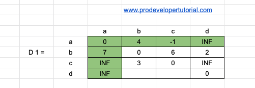
Similarly, we do it for [c, b] and [c, d].

1. [c to b]

Direct path value is = 3

Via “a” => c -> a + a -> b

Hence update 3.

2. [c to d]

Direct path value is INF.

Via “a” is c -> a + a -> d

Hence INF. Below are the updated values:

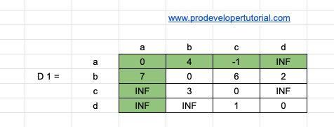
Similarly, we do it for [d, b] [d, c]

1. [d, b]

Direct path value is INF

Via “a” is => d -> a + a -> b

Update INF

2. [d, c]

Direct path value = 1

Via “a” is => d-> a + a-> c

Hence Min(1, INF). Update 1.

So D1 table is now completed. The result is as below:

Now from the above steps we can derive the formula to find out the min cost.

1 DK[i, j] = min [ Dk-1[i, j], Dk-1[i, k] + Dk-1[k, j] ]

Where k is the node number, D is the Distance matrix.

Now for the 2ndnode. Here K will be 2.

Now with the help of D1 matrix we construct D2 matrix.

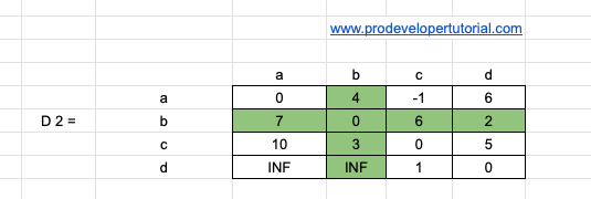
Now we shall take 2nd row and 2nd column from D1 matrix and copy into D2 matrix as below:

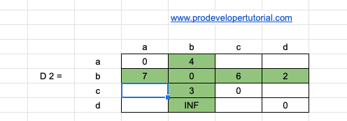
Similarly, like we did in D1 matrix, we take the min value of a direct path or the via path from “b”, and choose the min value. Here we shall take help of D1 matrix for reference.

1. [a, c]

Direct path value = -1

Via “b” path => a -> b + b ->c

As min is -1, choose -1.

2. [a, d]

Direct path value = INF

Via path value = “a -> b” + “b -> d”

Min[INF, 6] = 6

3. [c, a]

Direct path = INF

Via “b” path => “c->b” + “b -> a”

min[INF, 10] = 10

4. [c, d]

Direct path = INF

Via “b” path => “c->b” + “b->d”

min[INF, 5] = 5

5. [d, a]

Direct path = INF

Via “b” path = “d->b” + “b ->a”

6. [d, c]

Direct path = 1

Via path “d->b” + “b->c”

min(INF, 1) = 1

Hence the “D2” matrix will be as below

Now we shall construct “D3” matrix. Making row 3 and column 3 as constant by taking value from D2 matrix. The resultant matrix will be as below:

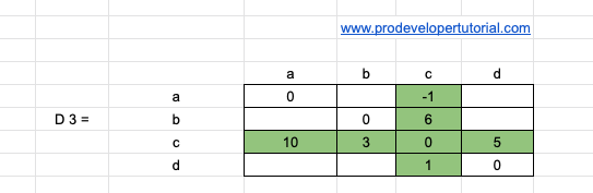
Again we calculate like above matrix. Now the via element will be “c”.

1. [a, b] => Direct path = 4,

min (4, 2) = 2

2. [a, d] => Direct path = 6,

min (6, 4) = 4

3. [b, a] => Direct path = 7,

min (16, 7) = 7

4. [b, d] => Direct path = 2,

min (11, 2) = 2

5. [d, a] => Direct path = INF,

min (INF, 11) = 11

6. [d, b] => Direct path = INF,

min (INF, 4) = 4

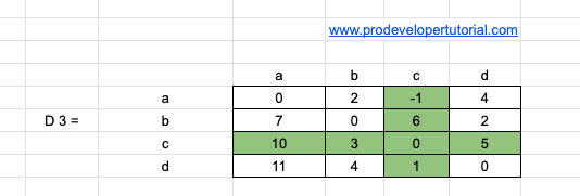
So the final matrix will be as below

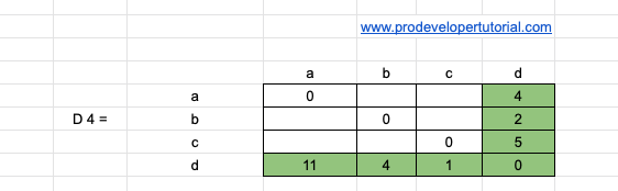
Similarly, we shall construct “D4” matrix. Initially we shall copy 4throw and 4thcolumn from “D3” matrix, and will look as below:

We shall calculate like above, the via element will be “d”.

1. [a, b] => Direct path = 2,

min (2, 8) = 2

2. [a, c] => Direct path = -1,

min (-1, 5) = -1

3. [b, a] => Direct path = 7,

min (7, 13) = 7

4. [b, c] => Direct path = 6,

min (6, 3) = 3

5. [c, a] => Direct path = 10,

min (10, 16) = 10

6. [c, b] => Direct path = 3,

min (3, 9) = 3

Finally we have completed calculating all the 4 matrices. The matrix “D4” will be the final matrix as below:

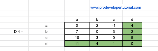
The above matrix will give the shortest path from any node to any other vertices.

#include<stdio.h>
#define V 4
#define INF 99999
 
void printSolution(int dist[][V]);
 
void floydWarshall (int graph[][V])
{
    int dist[V][V], i, j, k;
     for (i = 0; i < V; i++)
        for (j = 0; j < V; j++)
            dist[i][j] = graph[i][j];
 
    for (k = 0; k < V; k++)
    {
        for (i = 0; i < V; i++)
        {
            for (j = 0; j < V; j++)
            {
                if (dist[i][k] > dist[k][j] + dist[i][j])
                    dist[i][j] = dist[i][k] + dist[k][j];
            }
        }
    }
 
    printSolution(dist);
}
 
void printSolution(int dist[][V])
{
    printf ("The shortest distances"
            " between every pair of vertices \n");
    for (int i = 0; i < V; i++)
    {
        for (int j = 0; j < V; j++)
        {
            if (dist[i][j] == INF)
                printf("%7s", "INF");
            else
                printf ("%7d", dist[i][j]);
        }
        printf("\n");
    }
}
 
int main()
{
    int graph[V][V] = { {0,   5,  INF, 10},
                        {INF, 0,   3, INF},
                        {INF, INF, 0,   1},
                        {INF, INF, INF, 0}
                      };
 
    floydWarshall(graph);
    return 0;
}

---